Perlin noise

The purpose of this article is to describe the principle behind Perlin Noise the most intuitively possible, and explain how to implement it in practice. There are many ways to code Perlin Noise (some more optimized than others), but this article will focus on a simple and easily readable implementation.

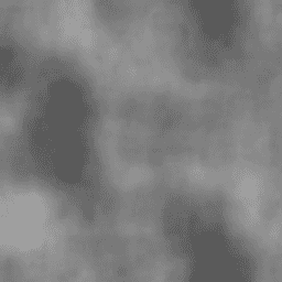
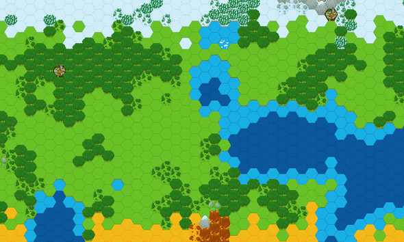
At the end, you will be able to produce a grayscale image generated using Perlin Noise, such as shown above. Of course, the algorithm can be used to produced other types of generated content, such as height maps. The hexagon map that you can see above was generated using 2 Perlin Noise maps: one for the elevation, and one for the forest.

The intuition behind Perlin Noise

The Perlin Noise algorithm can be summarized into the following steps:

• First, we divide our map into a grid of cells. At each intersection of the grid, we assign a gradient vector that will represent the slope of our final map this point. The figure below represents the grid of gradient vectors at each corner of our cells.

• To get the value of our Perlin Noise at a specific point, we first find the cell in which the point is contained.
• We then do some math magic: we compute the scalar product between each corner of the cell and the distance vector between this corner and our point.
• We interpolate the result of the 4 scalar products based on the position of our point in the cell.

This summary may sound complicated, but each step is detailed with code in the following sections. I give this summary so that you can have an overview of the progression of the algorithm.

The implementation

The goal of our algorithm is to produce a grayscale texture. For this, we will produce a 2-dimensional array of grayscale value ([0, 255] where 0 is black, and 255 is white), where each value represents a pixel, that we will fill thanks to Perlin Noise.

function get_grayscale_image(width, height, period) {
    let perlin_vectors = get_perlin_vectors(width, height, period);

    let pixels = new int[height][width]();

    for (let y = 0; y < height; y++) {
        for (let x = 0; x < width; x++) {
            let perlin_value = get_perlin_value(x, y, perlin_vectors, period);

            pixels[y][x] = 128 + 128 * perlin_value;
        }
    }

    return pixels;
}

We will implement the two functions get_perlin_vectors() and get_perlin_noise_grid() in the following sections. The first function will generate the grid of vectors used by the second function to compute the value of the point. Note that get_perlin_noise_grid() returns a value in the range [-1, 1], so we scale it so that it corresponds to a grayscale value in the range [0, 256].

Generate the gradient vectors

The goal is to generate a grid of cells, with a gradient vector at each intersection of the grid. We will compute the number of cells based on the size of the final image, and the size of a cell (which we will call period in the code).

function get_gradient_vectors(width, height, period) {
    let grid_width = Math.ceil(width / period) + 1;
    let grid_height = Math.ceil(height / period) + 1;

    let grid = new int[grid_height][grid_width]();
    for (let y = 0; y < grid_height; y++) {
        for (let x = 0; x < grid_width; x++) {
            grid[y][x] = random_vector();
        }
    }
}

You can do a quick sanity check to see if the formula for grid_width and grid_height are correct. For example, for a width of 7 and a period of 3, we will need 4 gradient vectors: one at 0, 3, 6 and 9.

There are multiple ways to implement the random_vector() function. For this article, we will simply generate a unit vector pointing in a random direction.

function random_vector() {
    let angle = random() * 2 * Math.PI;

    return {
        x: Math.cos(angle),
        y: Math.sin(angle),
    };
}

Note that I could have made the amplitude of the vector random too. This is up to you (and depending on the desired result) to choose which kind of method you want.

Retrieve the value at a certain point

Now comes the most mathematically intensive part. We are searching to get the Perlin Noise value at a certain coordinate (x, y). The entirety of the code presented in this section is placed inside a function:

function get_perlin_value(x, y, perlin_vectors, period) {
    // ...
}

We first determine which cell the point is in. For example, if we have a period of 3, and we want the Perlin value for the coordinate (3, 7), those calculations will yield cell_x = 1, cell_y = 2, relative_x = 0, relative_y = 0.33.

// Coordinate of the cell
let cell_x = Math.floor(x / period);
let cell_y = Math.floor(y / period);
// Relative coordinate of the point in the cell, normalized so that they are in [0, 1].
let relative_x = (x - cell_x * period) / period;
let relative_y = (y - cell_y * period) / period;

Before we proceed, we must apply a small smooth function over the relative coordinates. This will help round the edges of our Perlin noise, specially at the border of cells. In the interactive application at the end of the section, you will be able to toggle this application of the fade function to see its impact on the final result.

function fade(x) {
    return 6 * Math.pow(x, 5) - 15 * Math.pow(x, 4) + 10 * Math.pow(x, 3);
}

relative_x = fade(relative_x);
relative_y = fade(relative_y);

We will now fetch the 4 gradient vectors at the 4 corners of our cell.

let top_left_gradient = perlin_vectors[cell_y][cell_x];
let top_right_gradient = perlin_vectors[cell_y][cell_x + 1];
let bottom_left_gradient = perlin_vectors[cell_y + 1][cell_x];
let bottom_right_gradient = perlin_vectors[cell_y + 1][cell_x + 1];

We will now compute the 4 scalar products (also called dot product). The first 2 arguments represent the coordinates of the gradient vector of a corner and the last 2 represent the distance vector starting from this corner and to the point.

function dot(x1, y1, x2, y2) {
    return x1 * x2 + y1 * y2;
}

let top_left_contribution = dot(
    top_left_gradient.x,
    top_left_gradient.y,
    relative_x,
    relative_y
);
let top_light_contribution = dot(
    top_right_gradient.x,
    top_right_gradient.y,
    relative_x - 1,
    relative_y
);
let bottom_left_contribution = dot(
    bottom_left_gradient.x,
    bottom_left_gradient.y,
    relative_x,
    relative_y - 1
);
let bottom_right_contribution = dot(
    bottom_right_gradient.x,
    bottom_right_gradient.y,
    relative_x - 1,
    relative_y - 1
);

We now linearly interpolate (or lerp) the final value based on the 4 initial contributions. This means that we will give more weight to the top-left gradient if the point is closer to the top-left corner (this translates to a low relative_x and thus a high 1 - relative_x).

function lerp(a, b, t) {
    return a * (1 - t) + b * t;
}

let top_lerp = lerp(top_left_contribution, top_right_contribution, relative_x);
let bottom_lerp = lerp(
    bottom_left_contribution,
    bottom_right_contribution,
    relative_x
);
let final_value = lerp(top_lerp, bottom_lerp, relative_y);

return final_value / (Math.sqrt(2) / 2);

To get a final_value in the range [-1, 1], we must divide the final value by sqrt(2) / 2. Indeed, final_value will take its maximum value when the point is the center of the cell, and when the 4 corner gradients are directly pointing toward the point. In this specific configuration, the dot product will yield its maximum value which is the product of the amplitudes of the 2 vectors. Since our gradient vector always has an amplitude of 1 (see the random_vector function), and the distance between the center and the corner of a square whose sides are 1 in length is sqrt(2) / 2, the maximum value is 1 * sqrt(2) / 2 = sqrt(2) / 2. The lerp operations won’t influence this maximum value.

Here is a small simulator that implements the algorithm given above.

And here is the entire code in one block.

function dot(x1, y1, x2, y2) {
    return x1 * x2 + y1 * y2;
}

function lerp(a, b, t) {
    return a * (1 - t) + b * t;
}

function fade(x) {
    return 6 * Math.pow(x, 5) - 15 * Math.pow(x, 4) + 10 * Math.pow(x, 3);
}

function get_perlin_noise(x, y, period, perlin_vectors) {
    let cell_x = Math.floor(x / period);
    let cell_y = Math.floor(y / period);
    let relative_x = (x - cell_x * period) / period;
    let relative_y = (y - cell_y * period) / period;

    relative_x = fade(relative_x);
    relative_y = fade(relative_y);

    let top_left_gradient = perlin_vectors[cell_y][cell_x];
    let top_right_gradient = perlin_vectors[cell_y][cell_x + 1];
    let bottom_left_gradient = perlin_vectors[cell_y + 1][cell_x];
    let bottom_right_gradient = perlin_vectors[cell_y + 1][cell_x + 1];

    let top_left_contribution = dot(
        top_left_gradient.x,
        top_left_gradient.y,
        relative_x,
        relative_y
    );
    let top_light_contribution = dot(
        top_right_gradient.x,
        top_right_gradient.y,
        relative_x - 1,
        relative_y
    );
    let bottom_left_contribution = dot(
        bottom_left_gradient.x,
        bottom_left_gradient.y,
        relative_x,
        relative_y - 1
    );
    let bottom_right_contribution = dot(
        bottom_right_gradient.x,
        bottom_right_gradient.y,
        relative_x - 1,
        relative_y - 1
    );

    let top_lerp = lerp(
        top_left_contribution,
        top_right_contribution,
        relative_x
    );
    let bottom_lerp = lerp(
        bottom_left_contribution,
        bottom_right_contribution,
        relative_x
    );
    let final_value = lerp(top_lerp, bottom_lerp, relative_y);

    return final_value / (Math.sqrt(2) / 2);
}

The Perlin Noise at the moment doesn’t look good. To have something more visually appealing, we will need to implement Octaved Perlin Noise.

It is though interesting to see the impact of the parameters on the result. For example, if you set the period to 128 and disable smoothing, you will clearly the 16 cells (4 by 4) that makes the final image. By toggling the overlay, you can see the influence of the vectors on the color of the cell. The area in the direction of a gradient vector will generally be white, while the area “behind” a gradient vector will generally black.

Juxtaposing multiple octaves (or periods)

To get a good looking noise like shown in the first picture of this article, you must juxtapose multiple Perlin Noise with different periods. For example, we can take the noise with a period of 128, then 64, then 32, etc…

You may sometime see the term Octaved Perlin Noise when referring to this technique. In music, an octave is the interval between a period and its half (or a frequency, and its double).

To implement this, we simply re-generate multiple Perlin Noise grid with different periods, and linearly add them to form a merged grid. The code detailed in this section is contained in the following function:

function get_octaved_perlin_noise_grid(
    width,
    height,
    start_period,
    octaves,
    attenuation
) {
    // ...
}

We want to generate and merge octaves different grids. The first one will have a period of start_period, the second one a period of start_period / 2, the third one a period of start_period / 4 and so on.

We also want the small-period grids to have a lower impact on the final result than the big-period grids. Indeed, if you use your Perlin Noise to generate a heightmap (such as in Minecraft, for example), you want to use bigger periods to generate large mountains or large oceans, and smaller periods to generate small hills or pools. Note that you can always choose not to do that, depending on the result you want.

For this article, we will simply divide by 2 the range of the values for each octave. The first grid (period 128) will then yield values in the range [-1, 1], the second grid (period 64) in [-0.5, 0.5], the third grid (period 32) in [-0.25, 0.25] and so on. We say that we attenuate the higher octaves with a factor of 0.5. Note that we can generalize, and say that we attenuate the i-th octave by a factor of 0.5^i.

let final_grid = new int[height][width]();

for (let octave = 0; octave < octaves; octave++) {
    let period = start_period * Math.pow(1 / 2, octave);
    let octave_attenuation = Math.pow(attenuation, octave);

    let octave_grid = get_perlin_noise_grid(width, height, period);
    for (let y = 0; y < height; y++) {
        for (let x = 0; x < width; x++) {
            final_grid[y][x] += octave_grid[y][x] * octave_attenuation;
        }
    }
}

Note that since we add multiple grids together, we increase the maximum value that may be generated. Indeed, if we add 3 octaves together, with an attenuation of 0.5, final_grid may contain values up to 1 + 0.5 + 0.25 = 1.75. To be consistent with the first algorithm, we will compute this maximum value (max_value in the code) and divide every value of our grid by it, before finally returning the merged grid.

let max_value = 0;
for (let octave = 0; octave < octaves; octave++) {
    max_value += Math.pow(attenuation, octave);
}

for (let y = 0; y < height; y++) {
    for (let x = 0; x < width; x++) {
        final_grid[y][x] = final_grid[y][x] / max_value;
    }
}

return finalGrid;

Start by setting a period of 64 and only 1 octaves, you will see a traditionnal Perlin Noise like we did in the first part of this article. You can then increase the number of octaves and see the impact of each added Perlin Noise grid on the final image.

The entire code.

let final_grid = new int[height][width]();

for (let octave = 0; octave < octaves; octave++) {
    let period = start_period * Math.pow(1 / 2, octave);
    let octave_attenuation = Math.pow(attenuation, octave);

    let octave_grid = get_perlin_noise_grid(width, height, period);
    for (let y = 0; y < height; y++) {
        for (let x = 0; x < width; x++) {
            final_grid[y][x] += octave_grid[y][x] * octave_attenuation;
        }
    }
}

let max_value = 0;
for (let octave = 0; octave < octaves; octave++) {
    max_value += Math.pow(attenuation, octave);
}

for (let y = 0; y < height; y++) {
    for (let x = 0; x < width; x++) {
        final_grid[y][x] = final_grid[y][x] / max_value;
    }
}

return finalGrid;

Other uses

We saw how to generate a grayscale texture using Perlin Noise, but it can be used for many purposes.

To generate this map (thanks to @CuddlyColin for the assets), I used 2 Perlin Noise grids: one for the elevation to define water, land and mountain areas, and another one for the humidity to define land, forests and oasis. I had to tweak the numbers (periods, attenuation) a lot to get a good and natural map, this is why it is important to understand what impact each parameters has on the final result. You can for example guess that the period used for the Perlin noise will give a rough estimate of the size of an ocean or a forest in the final map.

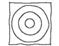
This image (Source) shows how you can Perlin Noise to simulate handwriting. The author generated a one-dimension Perlin Noise grid, and then, using a perfect circle as base, used it as an offset for the circle. Depending on the value on the noise, the circle will sometimes have a bigger radius, sometimes a lower radius, simulating a hand drawn circle.